

sommaire
I. Epreuve, loi binomiale et schéma de Bernoulli.
1.Epreuve de Bernoulli.
Soit p un nombre réel appartenant [O ; 1].
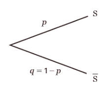
On appelle épreuve de Bernoulli toute expérience aléatoire n’admettant que deux issues, appelées
généralement succès S et échec  et de probabilités respectives et .
Exemples :
• Lancer une pièce de monnaie équilibrée et savoir si pile est obtenu est une épreuve de Bernoulli de succès S « Pile a été obtenu. » dont la probabilité est p = 0,5.
L’échec S est« Face a été obtenu. ».
• Interroger une personne dans la rue en France et lui demander si elle estgauchére
est une épreuve de Bernoulli de succès S « La personne est gauchère. » dont la
probabilité est .
2.Application et méthode sur les probabilités.
Exemple :
On tire une carte dans un jeu de 52 cartes. Pour chacune des épreuves suivantes, indiquer s’il s’agit d’une épreuve de Bernoulli et préciser le succès et sa probabilité le cas échéant.
1. On regarde la couleur de la carte (pique, coeur, carreau ou trèfle).
2. On vérifie que la carte est un pique.
3. On regarde si la carte n’est pas un pique.
4. On vérifie que la carte est un as.
5. On regarde la valeur de la carte (as, 2, 3, etc.).
6. On vérifie que la carte est une figure (roi, dame ou valet).
Solution :
1. Quatre issues sont possibles. Ce n’est pas une épreuve de Bernoulli.
2. II s’agit d’une épreuve de Bernoulli de succès « La carte est un pique. » dont la probabilité est .
3. II s’agit d’une épreuve de Bernoulli de succès « La carte n’est pas un pique. » dont la probabilité est .
4. II s’agit d’une épreuve de Bernoulli de succès« La carte est un as. » dont la probabilité est .
5. Treize issues sont possibles. Ce n’est pas une épreuve de Bernoulli.
6. II s’agit d’une épreuve de Bernoulli de succès « La carte est une figure. » dont la probabilité est .
3.La loi de Bernoulli.
On réalise une épreuve de Bernoulli dont le succès S a pour probabilité p.
Une variable aléatoire X est une variable aléatoire de Bernoulli lorsqu’elle est à
valeurs dans {0 ; 1} où la valeur 1 est attribuée au succès.
On dit alors que X suit la loi de Bernoulli de paramètre p.
Autrement dit, on et .
On peut résumer la loi de Bernoulli par le tableau suivant.
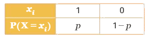
Soit X une variable aléatoire qui suit une loi de Bernoulli de paramètre p.
L’espérance mathématique de X est E(X) = p.
La variance de X est V(X)=p(1 —p).
Preuve :
L’espérance E(X) de X vaut :
La variance V(X) de X vaut :
4.Schéma de Bernoulli.
Soit n un nombre entier naturel non nul.
Un schéma de Bernoulli est la répétition de n épreuves de Bernoulli identiques et indépendantes.
Exemple :
On considère une urne opaque dans laquelle ont été placées une boule verte et deux boules bleues, toutes indiscernables au toucher. Et, on prélève une boule dans cette urne, on note sa couleur, puis on remet la boule dans l’urne. On répète ainsi dix fois l’expérience et on s’intéresse aux boules bleues obtenues. Chaque tirage est une épreuve de Bernoulli de succès S « La boule est bleue. » dont la probabilité est .
Comme les dix tirages se font avec remise, les tirages sont identiques et indépendants : on a bien un schéma de Bernoulli.
II. La loi binomiale.
1.Définition de la loi binomiale.
Soient n un entier naturel non nul et p un réel de l’intervalle [O ; 1].
On note X la variable aléatoire comptant le nombre de succès obtenu lors de n répétitions identiques et indépendantes d’un schéma de Bernoulli dont p est la probabilité du succès.
On dit alors que X suit la loi binomiale de paramètres n et p.
Soient k un entier naturel inférieur ou égal à n et X une variable aléatoire qui suit la
loi binomiale de paramètres n et p.
Alors
![]() .
.
Preuve :
Dans un schéma de Bernoulli, chaque chemin permettant d’obtenir k succès permet aussi
d’obtenir n- k échecs. Chacun de ces chemins a donc pour probabilité .
Chaque chemin est déterminé par la donnée de ses k succès : le nombre de chemins
menant à k succès est égal au nombre de combinaisons de k parmi n.
On en déduit que :
![]()
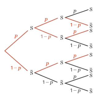
Illustration avec n = 3 :
En rouge les chemins menant à k = 2 succès.
Il y a 3 chemins permettant d’obtenir deux succès.
Chacun d’eux correspond à une probabilité égale à .
2. Représentation graphique de la loi binomiale.
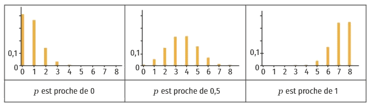
La représentation de la distribution correspondant à une loi binomiale dépend du paramètre p : plus p est proche de 0 et plus la probabilité d’obtenir un succès sera faible.
Si p devient proche de 1 alors la probabilité d’obtenir un grand nombre de succès sera élevée.
Ci-dessous, on voit ce qu’il se passe avec n = 8 et différentes valeurs de p.
La hauteur de chaque bâton au niveau de l’abscisse k correspond à P(X= k).
3. Espérance, variance et écart type.
Soient n un entier naturel strictement positif et p un nombre réel de l’intervalle [0 ; 1].
On note X une variable aléatoire qui suit la loi binomiale de paramètres n et p.
1. L’espérance de X est .
2. La variance de X est .
3. L’écart type de X est .
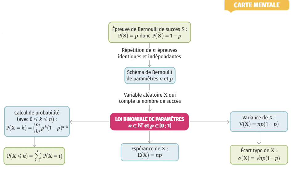
III. Carte mentale.


 Mathématiques Web c'est 2 208 412 fiches de cours et d'exercices téléchargées.